EEG analysis in Neutropic: resting state, ERP, ERD/ERS and SSVEP, step by step

EEG analysis usually lives in a script folder: MNE for filtering and epochs, a notebook for band power, another for the ERP figure, and a spreadsheet where the per-participant numbers end up before the statistics. Neutropic runs the same steps as seven deterministic EEG tools inside the chat. The language model decides which tool to call and writes the report, but every amplitude, latency and percentage comes from the tool, not from the model.

This post goes through EEG only, organised by study type. For the short tour across EEG, audio and video, see Beyond spreadsheets.

Shape the file first#

EEG goes in as a table (CSV, TSV or XLSX), one row per sample:

• Every numeric column is a channel, in µV. Name channels in the 10–20 system (Fp1, F3, Cz, Pz, O1 …). The names unlock topographic maps, frontal asymmetry and the C3/C4 lateralisation index.
• A `time_s` column lets the tools infer the sampling rate (from the median sample interval). If there is no time column, say the rate in your message ("sampled at 500 Hz").
• A `marker` column carries events: 0 on every sample without an event, a positive integer at the event onset sample. Each integer is a condition code (for example 1 = standard, 2 = target). ERP and ERD/ERS need it; resting-state and SSVEP analyses do not.

EDF, BDF or a vendor format? Convert it first. With MNE in Python, mne.io.read_raw_edf(path, preload=True) loads the file and raw.to_data_frame() gives a table with EEG already scaled to µV. Rename the time column to time_s, turn the annotations into integer codes with mne.events_from_annotations, write those codes into a marker column at the event samples, and save it as CSV. Drop EOG, ECG and trigger channels unless you want them treated as EEG.

Two ways to ask#

Type /eeg followed by your question. This sends the turn straight to the EEG tools. You can also describe the recording in plain words with /analyze. Either way, give the agent what the file cannot tell it: the paradigm, what each marker code means, and what you want reported.

The first tool is almost always eeg_info. It reports channels, sampling rate, duration, event counts per code, per-channel amplitude and flat-channel checks, and a line-noise ratio. If line noise is high or the peak-to-peak amplitude is large, the agent runs preprocessing before anything else.

Resting state: clean, band power, topography#

/eeg eeg_resting_10ch_250hz.csv is a 10-channel eyes-closed resting recording (250 Hz). Preprocess it (line-noise notch, band-pass, blink removal), compute band power per channel with an alpha topography, and report frontal alpha asymmetry (F4 vs F3) with figures.

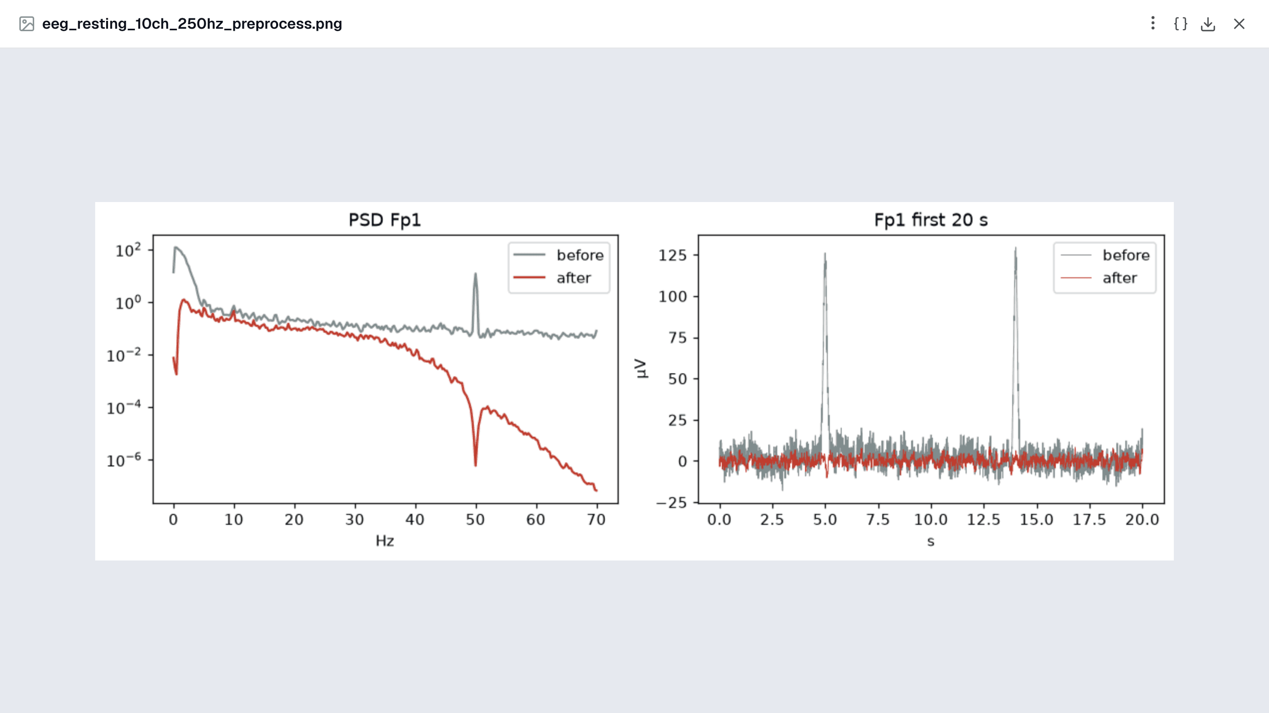
eeg_preprocess runs a fixed, visible pipeline:

• A 50 or 60 Hz notch (plus its harmonic), detected automatically.
• A 1–40 Hz zero-phase band-pass.
• An optional common average reference.
• FastICA blink removal.
• A pass that flags any 1-second window above 150 µV.

The cleaned data are saved as a new _clean.csv, and the original file is left untouched.

eeg_bandpower computes Welch band power per channel, in absolute (µV²) and relative (%) terms, for delta through gamma. It also gives the individual alpha peak, the theta/beta and theta/alpha ratios, and hemispheric asymmetry as ln(right) − ln(left). eeg_topomap draws each band on standard 10–20 positions.

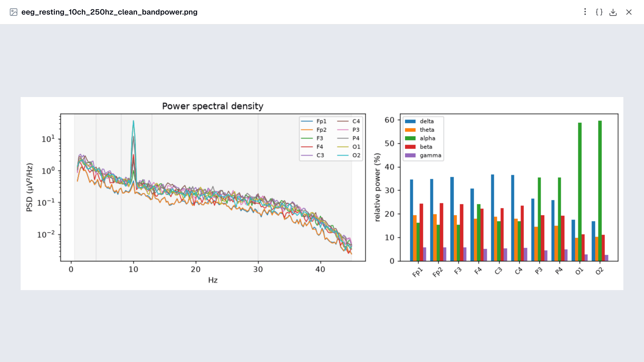
What came back on the sample recording. The sample was built with a 10 Hz occipital alpha, 50 Hz line noise, six blinks on Fp1/Fp2 and slightly more alpha at F4 than at F3. The line-noise ratio dropped from 37–58 to 0.0. ICA removed one component, which correlated 1.00 with the frontal channels. The alpha peak was 10.0 Hz on every channel, and relative alpha was highest at O2 (59.5%) and O1 (58.7%). F4 − F3 came out at +0.301. All of these match the simulated values.

What to check:

• The ICA line in the tool output: how many components were removed, and why (frontal correlation or kurtosis).
• The reference. Asymmetry depends on it, so eeg_bandpower recomputes it from the original reference even when you analyse an average-referenced file, and says which reference it used.
• The interpretation. The agent reads asymmetry only as relative frontal activation. It will not infer a personality or mood trait from one resting recording.

Event-related potentials: oddball P3#

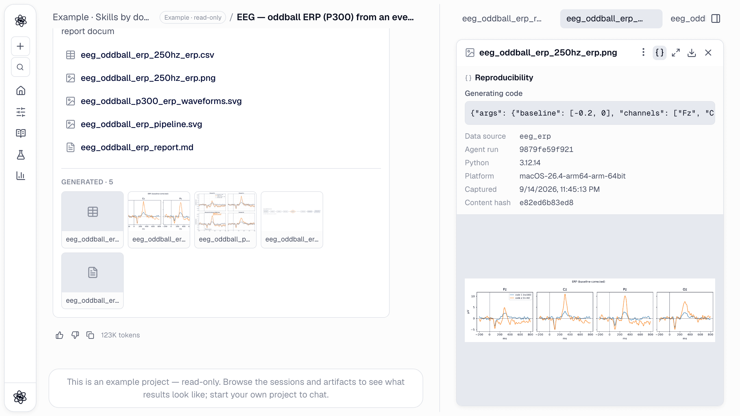
/eeg eeg_oddball_erp_250hz.csv is an auditory oddball recording (Fz, Cz, Pz, Oz; 250 Hz; marker 1 = standard, 2 = target). Epoch around the markers, baseline-correct, average per condition, report P3 latency and amplitude at Pz with the target-minus-standard difference wave, and plot the waveforms.

eeg_erp works through a fixed sequence:

• A 0.1–30 Hz filter.
• Epochs from −200 to 800 ms around each marker, with a pre-stimulus baseline.
• Rejection of any epoch that exceeds ±100 µV.
• An average per condition.

For every condition and channel it reports N1, P2, N2 and P3 peak latency, peak amplitude and window mean. It also gives the number of trials kept and rejected, a baseline noise SD and a P3 signal-to-noise ratio. With exactly two conditions it adds the difference wave. The averaged waveforms are saved as a CSV next to the figure.

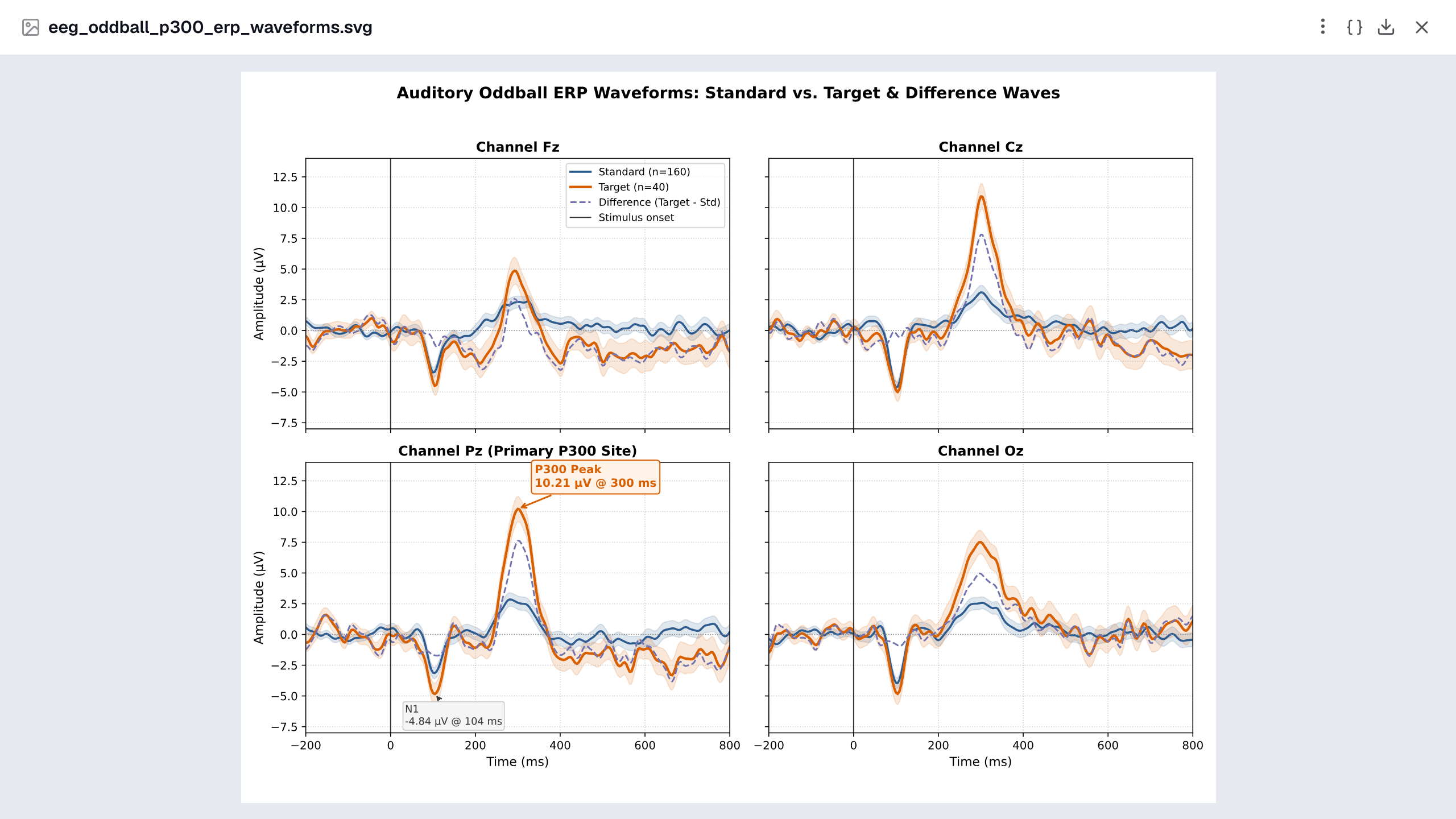
What came back. The sample had 160 standard and 40 target trials, a 100 ms N1 and a 300 ms P3 (12 µV target, 3 µV standard at Pz). All 200 epochs were kept. The target P3 at Pz peaked at 300 ms with 10.15 µV, the standard at 284 ms with 2.89 µV, and the difference wave at Pz was +7.58 µV. N1 appeared at about 104 ms. The latency is exact. The amplitude is slightly lower than simulated, as expected after the 0.1–30 Hz filter.

What to check:

• Trial counts per condition, and how many epochs were rejected.
• The component windows. They are fixed: N1 70–150 ms, P2 150–250 ms, N2 200–350 ms, P3 250–600 ms, each picked as the largest peak in its window. If your paradigm puts a component elsewhere, read the averaged-waveform CSV instead of the picked peak.
• The method paragraph against the recorded arguments. The report is written by the model. If its prose names a different filter or window from the one recorded for the tool call, the record is what actually ran.

Motor imagery: ERD/ERS#

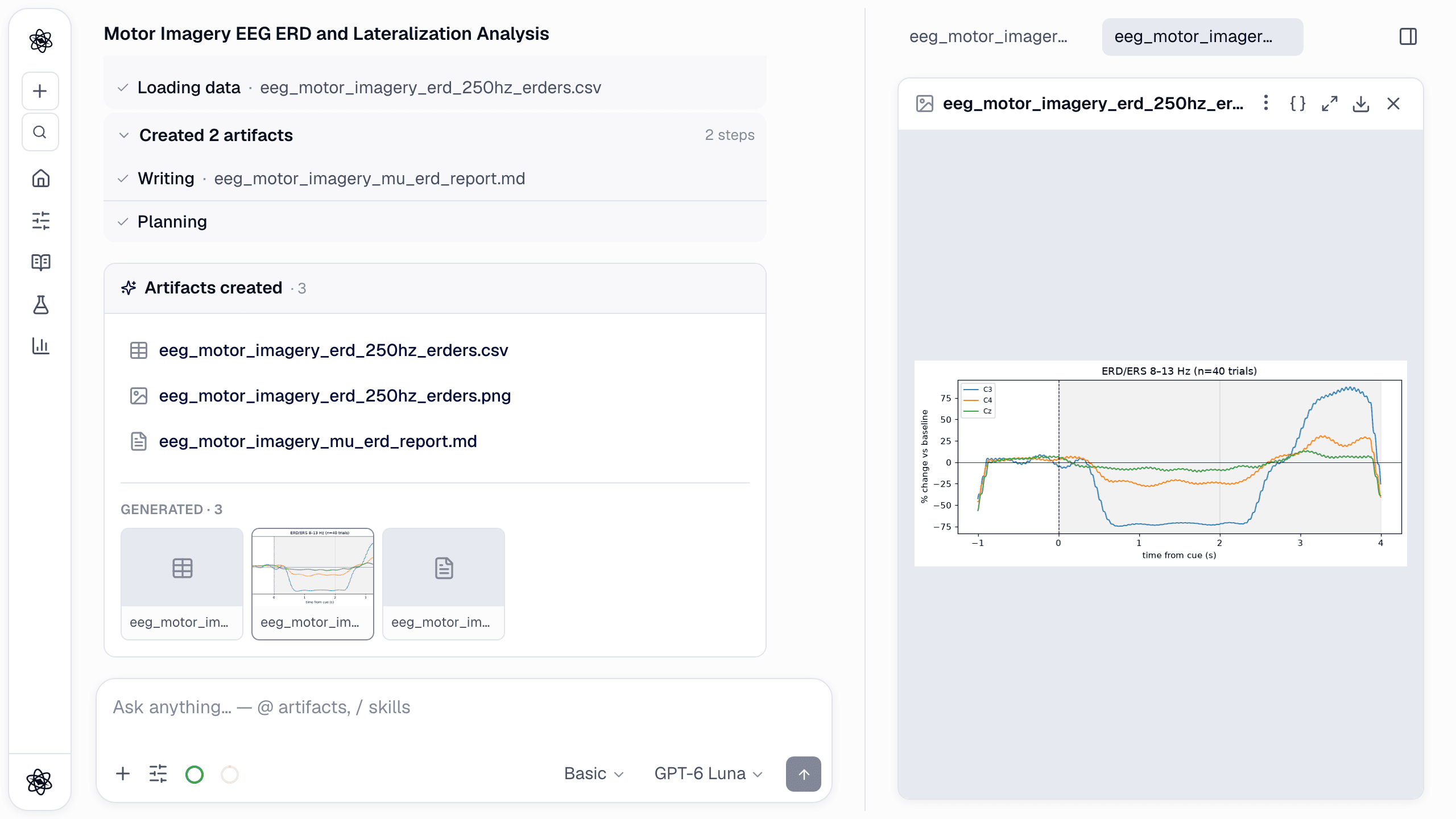
/eeg eeg_motor_imagery_erd_250hz.csv is a motor-imagery recording (C3, C4, Cz; 250 Hz; marker 1 = right-hand imagery cue, 40 trials). Compute mu-band (8–13 Hz) ERD/ERS against the pre-cue baseline, report ERD % during imagery and the rebound afterwards per channel, and check C3 vs C4 lateralisation.

eeg_erders band-passes the signal (mu 8–13 Hz by default, or any band you name), squares it and epochs around the cues. It then averages the trials, smooths with a 250 ms window and expresses power as % change from the baseline (Pfurtscheller & Lopes da Silva, 1999). Negative values are ERD and positive values are ERS. For each channel you get the ERD minimum and ERS maximum with their times and the mean % in each analysis window. When C3 and C4 are both present you also get a lateralisation index.

What came back. The sample was simulated with a C3 mu drop of about −75%, a weaker C4 drop and a rebound 3–4 s after the cue. In the English session the ERD minimum at C3 was −74.7% at 0.75 s, and the mean over 0–2 s was −54.7% at C3 versus −16.9% at C4. The rebound peaked at +88.0% at 3.62 s, and the lateralisation index was 0.53, with C3 stronger, as expected for right-hand imagery.

What to check:

• The windows and the baseline. The tool's defaults are a −1 to 5 s epoch and windows of 0.5–2.5 s and 3–4 s. In this session the agent chose 0–2 s and 2–4 s and said so in the report. Window means are only comparable across recordings when you fix the windows in your prompt.
• Epoch edges. A minimum that lands on the last sample of the epoch is an edge effect, and the report flagged exactly that for C4 and Cz.
• Trial statistics. These are trial-averaged values from one recording, with no trial-level uncertainty.

SSVEP: which frequency was attended#

/eeg eeg_ssvep_12hz_250hz.csv is a 20 s SSVEP recording (O1, Oz, O2, Cz; 250 Hz). The candidate flicker frequencies were 8.57, 10, 12 and 15 Hz. Decide which one was attended, report CCA ρ and SNR for every candidate, and check the decision in 4 s windows.

eeg_ssvep band-passes 3–60 Hz, then scores every candidate frequency in two independent ways:

• CCA: canonical correlation with sine/cosine references, including harmonics (Lin et al., 2006).
• SNR: spectral power at the frequency relative to its neighbours.

It reports whether the two methods agree. With a window length it also repeats the decision per window and gives the agreement rate.

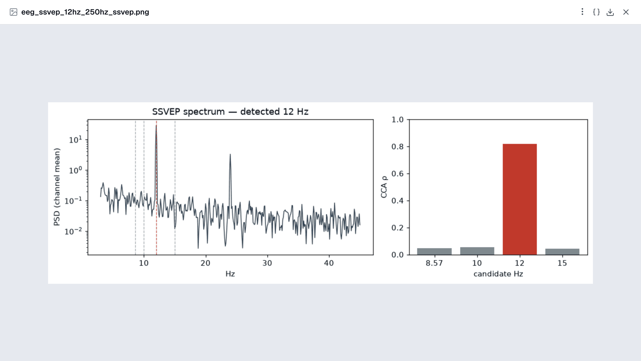
What came back. The sample was a 12 Hz stimulus with a 24 Hz harmonic. The detected frequency was 12 Hz, with CCA ρ 0.82 and 22.9 dB SNR. Every other candidate had ρ ≤ 0.055. All five 4 s windows agreed, for 100% agreement.

What to check: the full candidate table, not just the winner. A winner with a small ρ margin over the runner-up, or disagreement between CCA and SNR, is a weak decision.

From per-recording numbers to statistics#

The EEG tools work on one recording at a time. A study needs one row per participant, for example P3 amplitude at Pz per participant and group. Run the tool per file, or ask the agent to collect the values into one table, then hand that table to the statistics skill:

/stats Compare P3 amplitude at Pz between the patient and control groups in p3_by_participant.csv. Check the assumptions, choose the test and explain why.

compare_groups identifies the design, checks normality and variance, and picks the test by rule. For example, it uses Welch when variances differ and Mann–Whitney for small, non-normal samples. It returns an effect size with a CI and a decision trace that explains the choice. Repeated conditions within participants (target vs standard) go to paired tests or repeated-measures designs, and nested trial-level data can go to a mixed model. More in the statistics walkthrough.

Every sentence traceable, every figure reproducible#

After the turn, Neutropic adds sentence-level [n] citations to the analysis report. Each [n] points to one analysis step from that turn (a tool call with its output) or to the data file, and the reference list at the end names them. When a number looks surprising, you can open the step it came from.

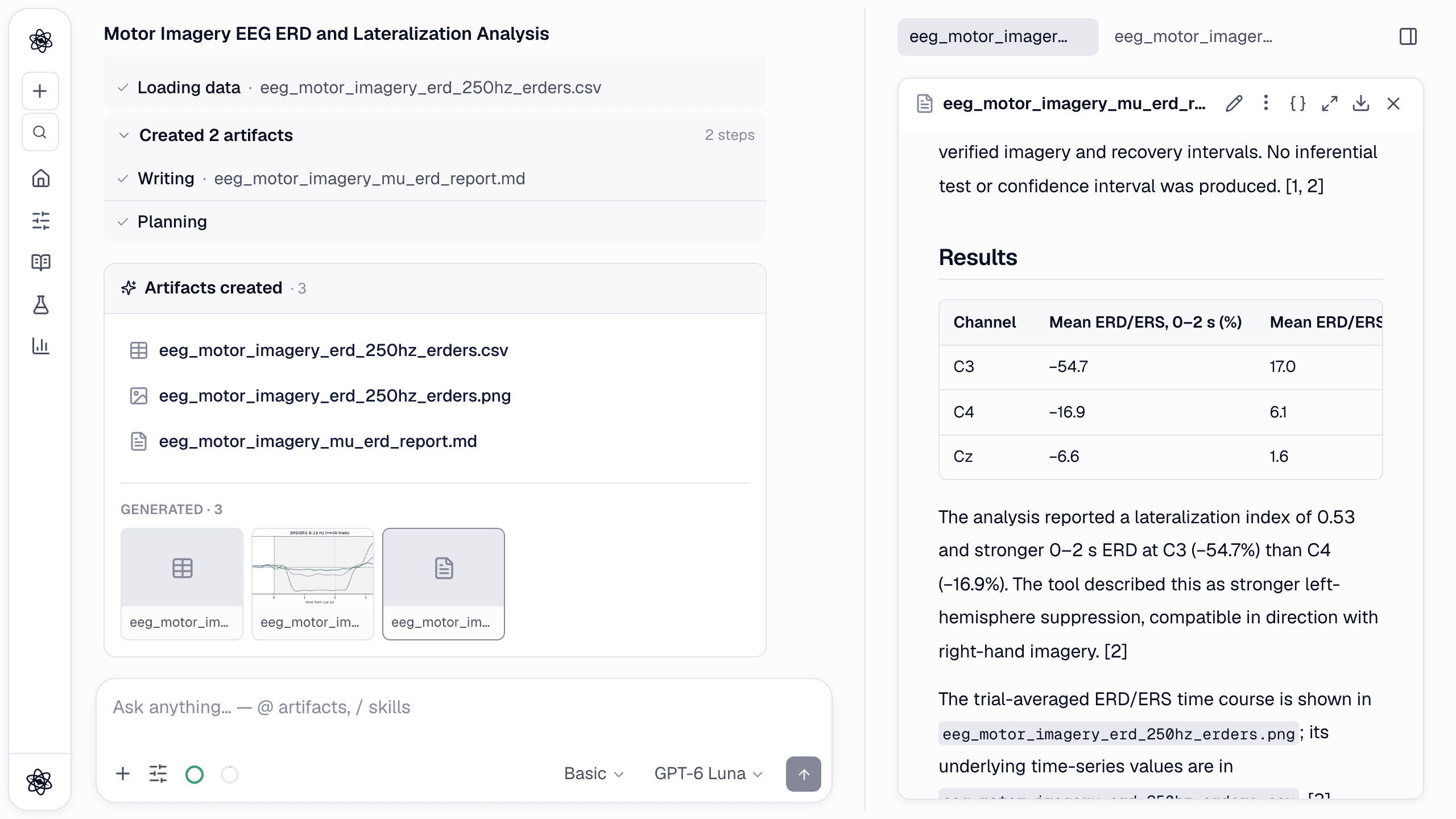
Every figure and table records the tool and the exact arguments that produced it. Press { } in the artifact panel to see them. Cleaned data are saved as new files, so the raw recording is never overwritten. More in Every sentence cited and Reproducibility by default.

Honest limits#

• Input. Tables only. EDF, BDF and vendor formats need converting. Amplitudes are assumed to be µV, and the sampling rate is assumed to be uniform.
• Blink removal. It needs frontal channels (Fp1/Fp2, AF*, F7/F8), because separate EOG channels are not used. Without frontal channels, blinks are not removed. Windows over threshold are flagged, not cut out.
• Topographies. They use standard 10–20 positions, not digitised electrode locations. They need at least three recognised 10–20 names, and other channels are left out of the map.
• ERP. The component windows are fixed. The difference wave is computed only for exactly two conditions. The figure shows the first four channels, and the CSV holds all of them.
• ERD/ERS and SSVEP. Results are trial-averaged or whole-recording, with no trial-level statistics. SSVEP uses standard CCA with sine/cosine references and needs the candidate frequencies from you. Individual-template or filter-bank variants are not included.
• The report. It is written by the model from the tool outputs. The numbers come from the tools, but check its method prose against the recorded arguments.

Open Example · Skills by domain to see the resting-state and ERP sessions, or attach your own recording and type /eeg. For the full walkthrough of physiological recordings beyond EEG, see Neutropic for psychophysiology labs.